Teaching Time Series in the Covid-affected Era
All time-series forecasting methods make their forecasts by taking patterns from the past and projecting them into the future. (And there are lots of different methods for doing this.)
Because all we can do is project from the patterns we already have seen, when unprecedented patterns emerge (i.e., patterns we have never seen before), our forecasting methods fail. This is an unavoidable reality. Short of clairvoyance, it couldn’t be any other way. It is impossible for the projected trends and confidence limits our tools produce to make reasoned allowances for types of changes we have never before experienced or thought about. In the context of our experience they are unexpected outliers.
Some series, especially tourism related, have reacted to covid-19 by producing patterns we have never seen before. For those situations the forecasts from our simple Year-13 tools fail. All the assumptions that have been used in making their forecasts have been violated by emerging real-world events. Currently (January 2021) , for example, even the professionals have no idea of how to reliably forecast what will happen to visitor arrivals in New Zealand over the next year or two. They have no real idea what the pattern of recovery will look like over what period.
There are a lot of other data series for which covid has had next to no effect (e.g., climate series), or little effect (e.g., fruit and vegetable prices as in Figure 5 below). Our current tools work fine for those.
At year 13 our students learn to work with time series that show a particular, visually-obvious, type of pattern that is quite common, a trend plus a regularly repeating seasonal component (cf. Figure 2 below).
It is important for students to see series that do look like this (and for which our tools are appropriate), and others that do not (and for which our tools are not appropriate). We recommend that formal NCEA assessments use the former type of series, but that students are shown examples of both and can distinguish between them. We give some illustrative examples after the following set of links. We conclude with descriptions of some methods that professionals use to cope with disruptions in time series.
If you are unfamiliar with these ways of thinking and working, or if you want a reminder, see the following short videos [mins: secs]:
- Introducing Time Series [4:38]
- Seasonal Decomposition & Forecasting, Part I [6:01]
- Seasonal Decomposition & Forecasting, Part II [5:12]
- A simple but interesting extension: Comparing Series [5:16]
These are also on https://new.censusatschool.org.nz/resources/3-8/ under “Teacher Preparation” together with pdfs that contain illustrated transcripts of what the movies say.
Examples
Figure 1 below shows monthly time-series data of average numbers of overseas visitors in NZ from January 2010 until December 2020.
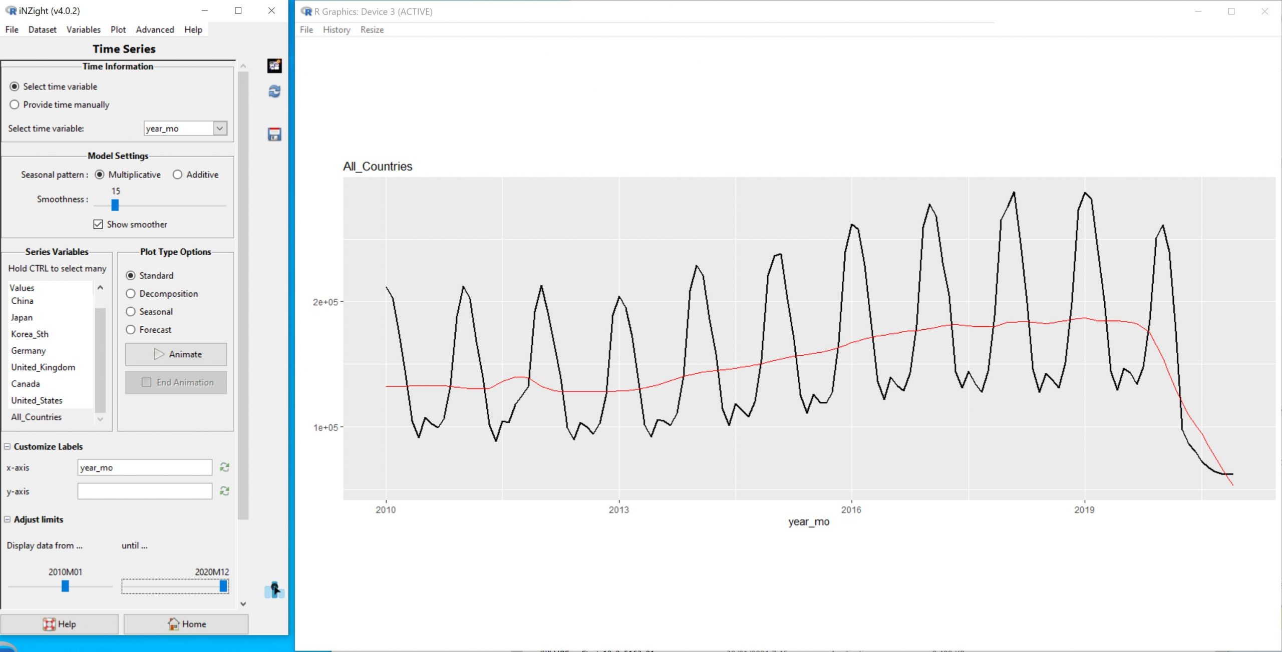
Figure 1: Monthly series of average overseas visitors in NZ from January 2010 until December 2020
Figure 2 shows a seasonal decomposition of this series using just the data up until January 2020. The thin blue line shows an estimated trend plus a repeating seasonal effect. It almost perfectly reproduces the actual data (red line). (Note: few series are this perfectly modelled by a trend plus seasonal effect). But after January 2020 covid starts to affect things, borders get closed and visitor numbers begin to fall off a cliff. The simple analysis tools we give our students cannot cope with this radical change in behaviour.
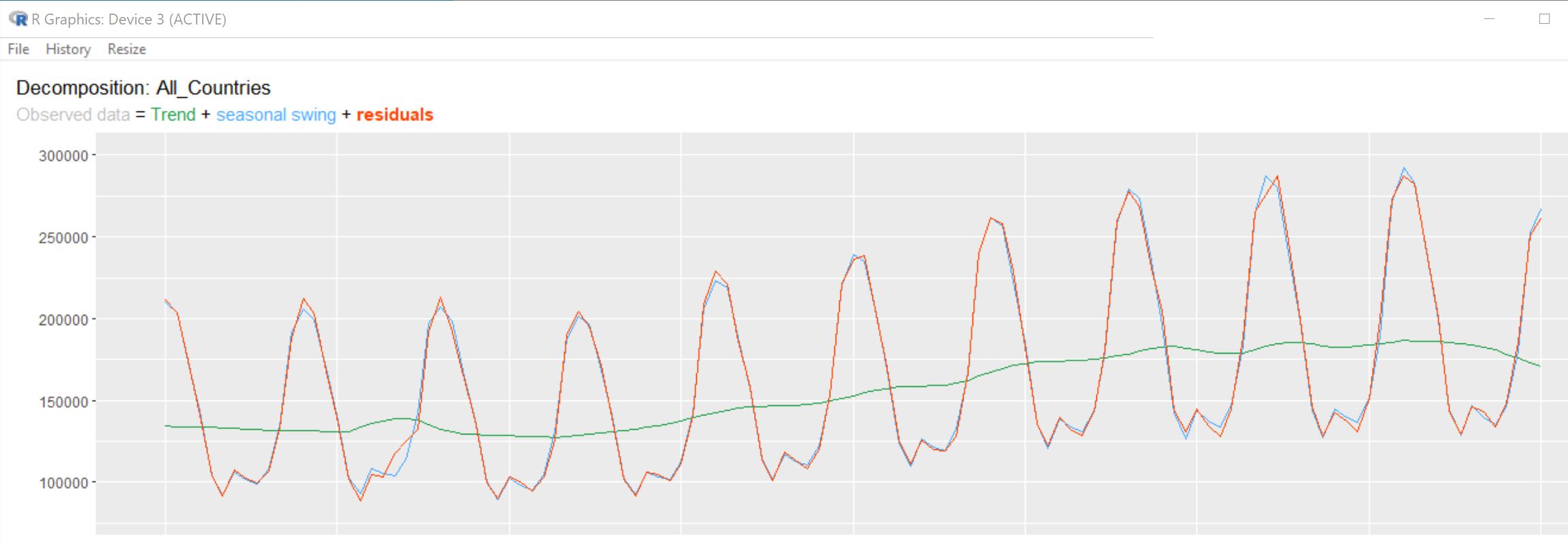
Figure 2: Decomposition of this series from January 2010 to January 2020
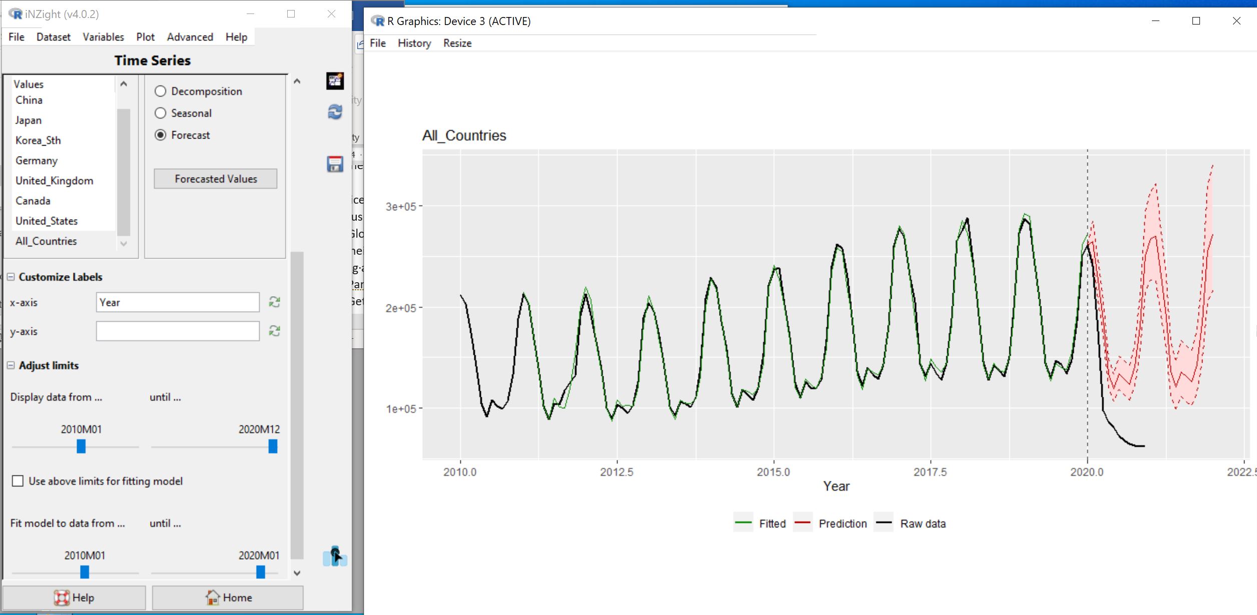
Figure 3: Forecasting visitor numbers after January 2020 using the data from 2010-January 2020
Figure 3 uses the data up to January 2020 to forecast average visitor numbers from February 2020 on. We see the forecast (red line) with its uncertainty bands in pink. The actual data is the black line. The forecast missed what really happened by miles. Our forecasts are made by projecting forwards the patterns we have seen in the past but, in 2020, covid and border closures changed everything and the real series departed from the patterns it had followed in the past and started behaving in a way that we had never seen before.
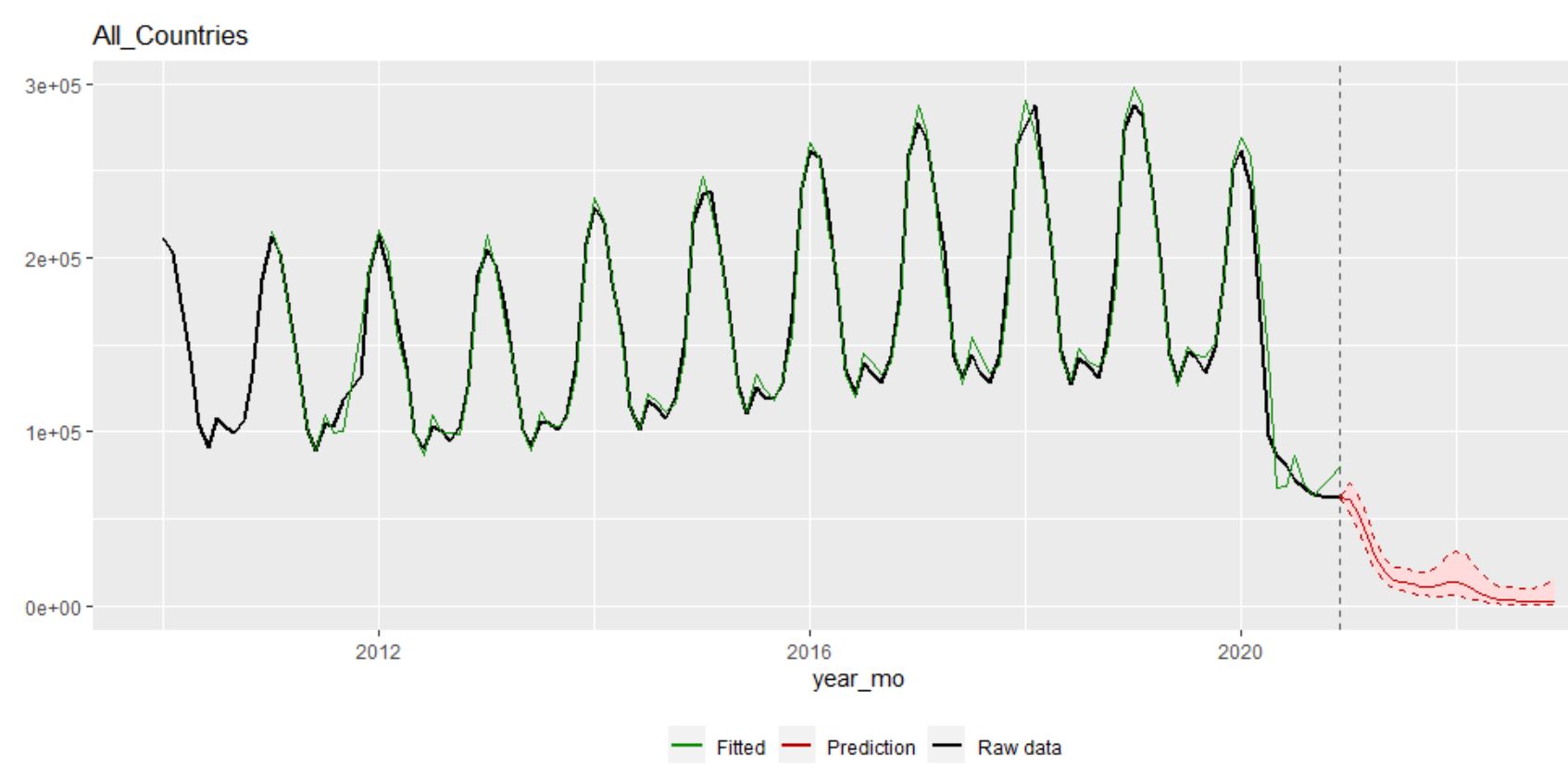
Figure 4: Forecasting visitor numbers in 2021 and beyond using the data up until December 2020
Figure 4 tries to forecast 2021 and beyond using all the data up until December 2020. We cannot trust this forecast at all because the simple (monotone) trend plus season model the Holt-Winter method is assuming is no longer applicable. The pattern has been broken and we don’t know if, when, and over what period it might “go back to normal”. Students should see this and learn a very big lesson about forecasting from it — that the world doesn’t always play nice with us and sometimes something new and unexpected happens that makes our forecasts badly wrong.
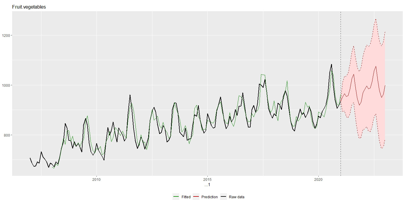
Figure 5: Forecasting average fruit and vegetable price index values using data up until December 2020
Figure 5 is looking at the fruit and vegetable component of the NZ consumer price index (CPI) up until December 2020 and doing a Holt-Winters forecast for 2021 and 2022. Looking at the historical data (black line) and how it is approximated by the Holt-Winters modelled trend+seasonal-effect estimates (green line) you will see that there is nothing particularly unusual about 2020. We could use this series in an assessment.
But as we have said professionals can do better at modelling and forecasting time series than we can because they have a wider range of tools. Professional times-series analysts have methods for making adjustments for all sorts of strange behaviours.
Modelling for disrupted time series
By Rachel Passmore
[Note: this is beyond the scope of NCEA Level 3]
Disruptions to time series are a relatively common event for time series modellers to contend with. Disruptions may be caused by price changes, policy changes, definition changes and environmental changes as well as pandemics. Recovery from such disruptions can be handled in a number of ways, depending on what information about the disruption is available. For example, if a time series has been disrupted by a price change, there may have been other price changes in the past, so an estimate of the impact of a price change can be made and the time taken for levels to recover can be made and projections adjusted accordingly. The four most common patterns for a disruption are:
- Permanent shift to the level of the time series, either up or down.
- A ‘blip’ , perhaps caused by a one-off event; time series resumes pre-blip level and patterns afterwards.
- Permanent shift to the level of the time series but it does not happen all at once.
- Sudden shift to the level of the time series which gradually over time reverts to its pre-sudden shift level
Each of these possibilities can be incorporated into a model of time series. This part of time series analysis is known as intervention analysis and is usually modelled using an ARIMA or Autoregressive Integrated Moving Average Model although other models are possible too. Some disruptions to time series are not easy to detect, and this is where change point detection can be employed. This technique can be used to detect sudden changes in live data streams for monitoring purposes, but can also be used to detect all historic changes in the time series, not just the most obvious one
Some Australian researchers have also been developing probabilistic forecasting. They were interested in forecasting international arrivals to Australia as there is strong interest from a number of parties in knowing when pre-COVID levels might resume, if ever. Their approach was to survey 433 tourism experts and ask their opinion on pessimistic, most-likely and optimistic rates of recovery in visitor arrivals. Scenario-based
Probabilistic forecasts were produced and compared with forecasts generated as though COVID had never happened. This allowed tourism operators to estimate the difference between the scenario-based probabilistic forecasts and the projections generated as if the pandemic had never occurred.
Intervention analysis and scenario-based probabilistic forecasting iis beyond the scope of the NZ Secondary School curriculum, but given the number of time series data sets that could be impacted by the pandemic, here are some suggestions that could provide a way forward, admittedly they are a bit of a ‘fudge’ !
- Permanent shift to level of time series. In this instance, remove data post shift and predict from the last pre-shift data point. Make an assumption about the size of the shift, and reduce/increase projections by that amount.
- Blip – remove this value from the data set and replace with an interpolated value, then calculate projections in the usual manner
- Permanent shift that happens over time, such as a gradual decline. This could be be modelled by adding an additional variable in the model that decreases over time.
- Sudden shift that gradually recovers to pre-disruption levels. This could be modelled by adding an additional variable in the model that increases over time until pre-disruption levels are regained.
The first scenario can be handled by employing iNZight in the usual way, but then adjusting projections by the estimated size of the shift. At secondary school level, this does not have to be a sophisticated estimate; as long as some justification can be provided for the size of the estimate that should be sufficient.
The second scenario just requires substitution of the one unusual data value, then iNZight can be used in the usual way.
The third scenario requires two assumptions to be made; the size of the shift, and the length of time taken for the shift in mean level to occur. This is definitely outside the scope of secondary school students in terms of assessment, but might be a useful teaching activity to discuss how this could be done. Suggestions include taking projections produced by data up to but not including any COVID effect, and then adjusting projections by applying a linear or non-linear decay element.
The fourth scenario can be handled in a similar fashion to the third scenario, but this time adjust projections by applying a growth element for a limited period of time.
References
https://link.springer.com/referenceworkentry/10.1007%2F978-3-642-04898-2_308
https://online.stat.psu.edu/stat510/lesson/9/9.2
https://www.monash.edu/business/ebs/research/publications/ebs/wp01-2021.pdf